
Matplotlib(基礎編)
Contents
Matplotlib(基礎編)#
![]()
まずは、Chainerチュートリアル通りプロット。 簡単なグラフはこれで十分です。
ここでは、numpyでデータを作成しつつプロットを行います。
import numpy as np
import matplotlib.pyplot as plt
numpyの使い方#
一定区間に等間隔で散らばった点を生成
np.arange(開始, 終了, 間隔)
x = np.arange(-1, 1, 0.1)  # -1から1まで、0.1刻みで点を生成する

x
array([-1.00000000e+00, -9.00000000e-01, -8.00000000e-01, -7.00000000e-01,
       -6.00000000e-01, -5.00000000e-01, -4.00000000e-01, -3.00000000e-01,
       -2.00000000e-01, -1.00000000e-01, -2.22044605e-16,  1.00000000e-01,
        2.00000000e-01,  3.00000000e-01,  4.00000000e-01,  5.00000000e-01,
        6.00000000e-01,  7.00000000e-01,  8.00000000e-01,  9.00000000e-01])
関数にわたす
np.arrayを関数に渡すと、その要素全てに同じ操作が加えられます。
例)
np.array([1, 2, 3]) ** 2

# array([1, 4, 9])
その他、numpyで定義されている関数
sincostanlogexp
も使えます。
y = np.sin(x)  # 生成した点をsin関数に渡す

y
array([-8.41470985e-01, -7.83326910e-01, -7.17356091e-01, -6.44217687e-01,
       -5.64642473e-01, -4.79425539e-01, -3.89418342e-01, -2.95520207e-01,
       -1.98669331e-01, -9.98334166e-02, -2.22044605e-16,  9.98334166e-02,
        1.98669331e-01,  2.95520207e-01,  3.89418342e-01,  4.79425539e-01,
        5.64642473e-01,  6.44217687e-01,  7.17356091e-01,  7.83326910e-01])
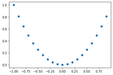
散布図#
plt.scatter(xの配列, yの配列)
平面状に点を打ちます。
x = np.arange(-1, 1, 0.1)
y = x ** 2

plt.scatter(x, y)
<matplotlib.collections.PathCollection at 0x10f6fbe50>
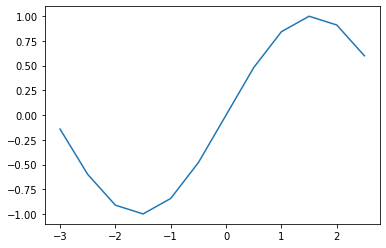
折れ線グラフ#
plt.plot(xの配列, yの配列)
散布図と異なり、隣り合った点をつなげます。
x = np.arange(-3, 3, 0.5)
y = np.sin(x)

plt.plot(x, y)
[<matplotlib.lines.Line2D at 0x10f83ea40>]
ヒストグラム#
データの生成
\(1〜6\) までの数字をランダムに \(1000\) 回選んで平均を求めます。
これを \(1000\) 回繰り返して、どんな分布になっているかをみてみます。
from random import randint

data = []

for i in range(1000):

    # 1~6までの数字をランダムに選んで足す x 1000回
    sum_of_dice = 0
    for j in range(1000):
        sum_of_dice += randint(1, 6)

    ave_of_dice = sum_of_dice / 1000  # 1000で割って平均を出す
    data.append(ave_of_dice)


print(data[:10])  # 10個目までを見る
[3.558, 3.477, 3.442, 3.517, 3.477, 3.541, 3.454, 3.475, 3.526, 3.423]
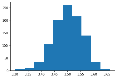
ヒストグラムを作成
plt.hist(データ)
自動的に階級の幅を決めてプロットしてくれます。 この場合は \(10\) 個の階級に分けられていました。
plt.hist(data)
(array([  5.,   9.,  32., 104., 201., 259., 215., 138.,  32.,   5.]),
 array([3.301 , 3.3371, 3.3732, 3.4093, 3.4454, 3.4815, 3.5176, 3.5537,
        3.5898, 3.6259, 3.662 ]),
 <BarContainer object of 10 artists>)
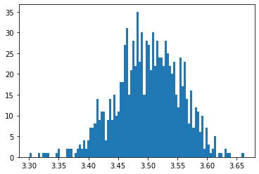
パラメータの調整#
hist関数にオプションで bins=100 を渡すと、階級を \(100\) 個に分けることができます。
plt.hist(data, bins=100)
(array([ 1.,  0.,  0.,  0.,  1.,  0.,  1.,  1.,  1.,  0.,  0.,  0.,  1.,
         2.,  0.,  0.,  0.,  2.,  2.,  2.,  0.,  1.,  2.,  3.,  2.,  4.,
         2.,  4.,  7.,  7.,  8., 14.,  9., 11., 11.,  4.,  9., 14.,  9.,
        15., 10., 11., 18., 18., 27., 31., 15., 21., 28., 22., 35., 23.,
        30., 15., 28., 27., 21., 30., 22., 28., 24., 24., 22., 28., 25.,
        22., 20., 23., 15., 12., 24., 17., 23., 14.,  8., 16.,  7., 12.,
        11.,  6., 10.,  2.,  7.,  3.,  1.,  2.,  5.,  0.,  1.,  1.,  0.,
         2.,  1.,  1.,  0.,  0.,  0.,  0.,  0.,  1.]),
 array([3.301  , 3.30461, 3.30822, 3.31183, 3.31544, 3.31905, 3.32266,
        3.32627, 3.32988, 3.33349, 3.3371 , 3.34071, 3.34432, 3.34793,
        3.35154, 3.35515, 3.35876, 3.36237, 3.36598, 3.36959, 3.3732 ,
        3.37681, 3.38042, 3.38403, 3.38764, 3.39125, 3.39486, 3.39847,
        3.40208, 3.40569, 3.4093 , 3.41291, 3.41652, 3.42013, 3.42374,
        3.42735, 3.43096, 3.43457, 3.43818, 3.44179, 3.4454 , 3.44901,
        3.45262, 3.45623, 3.45984, 3.46345, 3.46706, 3.47067, 3.47428,
        3.47789, 3.4815 , 3.48511, 3.48872, 3.49233, 3.49594, 3.49955,
        3.50316, 3.50677, 3.51038, 3.51399, 3.5176 , 3.52121, 3.52482,
        3.52843, 3.53204, 3.53565, 3.53926, 3.54287, 3.54648, 3.55009,
        3.5537 , 3.55731, 3.56092, 3.56453, 3.56814, 3.57175, 3.57536,
        3.57897, 3.58258, 3.58619, 3.5898 , 3.59341, 3.59702, 3.60063,
        3.60424, 3.60785, 3.61146, 3.61507, 3.61868, 3.62229, 3.6259 ,
        3.62951, 3.63312, 3.63673, 3.64034, 3.64395, 3.64756, 3.65117,
        3.65478, 3.65839, 3.662  ]),
 <BarContainer object of 100 artists>)
箱ひげ図#
データの生成
確率90%、60%、30%で表が出るコインを用意して、何回連続で表が出るかを調べます。
それぞれ1000回ずつ試行します。
from random import randint
prob_90 = []
prob_60 = []
prob_30 = []

for i in range(1000):

    # 90%が何回連続で出るか
    count_90 = 0
    while randint(1, 100) <= 90:
        count_90 += 1
    prob_90.append(count_90)

    # 60%が何回連続で出るか
    count_60 = 0
    while randint(1, 100) <= 60:
        count_60 += 1
    prob_60.append(count_60)

    # 30%が何回連続で出るか
    count_30 = 0
    while randint(1, 100) <= 30:
        count_30 += 1
    prob_30.append(count_30)

print("90%: ", prob_90[:20])
print("60%: ", prob_60[:20])
print("30%: ", prob_30[:20])
90%:  [0, 3, 12, 10, 18, 10, 3, 0, 0, 1, 2, 13, 16, 13, 0, 26, 0, 3, 28, 6]
60%:  [0, 2, 0, 0, 1, 0, 0, 1, 0, 3, 0, 0, 3, 0, 1, 0, 0, 0, 5, 0]
30%:  [1, 0, 1, 1, 4, 1, 1, 1, 0, 0, 0, 0, 1, 0, 0, 0, 1, 0, 0, 0]
plt.boxplot((prob_90, prob_60, prob_30))
{'whiskers': [<matplotlib.lines.Line2D at 0x10fa88730>,
  <matplotlib.lines.Line2D at 0x10fa88a00>,
  <matplotlib.lines.Line2D at 0x10fa89ae0>,
  <matplotlib.lines.Line2D at 0x10fa89db0>,
  <matplotlib.lines.Line2D at 0x10fa8ae90>,
  <matplotlib.lines.Line2D at 0x10fa8b160>],
 'caps': [<matplotlib.lines.Line2D at 0x10fa88cd0>,
  <matplotlib.lines.Line2D at 0x10fa88fa0>,
  <matplotlib.lines.Line2D at 0x10fa8a080>,
  <matplotlib.lines.Line2D at 0x10fa8a350>,
  <matplotlib.lines.Line2D at 0x10fa8b430>,
  <matplotlib.lines.Line2D at 0x10fa8b700>],
 'boxes': [<matplotlib.lines.Line2D at 0x10fa88460>,
  <matplotlib.lines.Line2D at 0x10fa89810>,
  <matplotlib.lines.Line2D at 0x10fa8abc0>],
 'medians': [<matplotlib.lines.Line2D at 0x10fa89270>,
  <matplotlib.lines.Line2D at 0x10fa8a620>,
  <matplotlib.lines.Line2D at 0x10fa8b9d0>],
 'fliers': [<matplotlib.lines.Line2D at 0x10fa89540>,
  <matplotlib.lines.Line2D at 0x10fa8a8f0>,
  <matplotlib.lines.Line2D at 0x10fa8bca0>],
 'means': []}
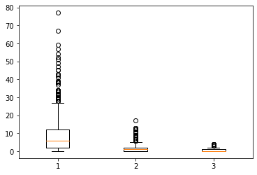
90%だと70回以上出ることもあるのに対して、 30%だと10回以上連続で出ることはほとんどないですね。